Main nonlinear dynamic modes of climate variability

According to eq. (1), the main objective of the proposed expansion is to decompose multivariate time series (distributed in space) made up of points X(t_m): = X^m into a set of main modes, each of them is represented by a one-dimensional parametric curve . Below, we briefly state the main points of the method we propose; more technical details can be found in the additional methods.

bayesian reconstruction

As in the traditional EOF decomposition, we use a recursive procedure for a successive reconstruction of the terms (modes) in the equation. (1). The first step is to find the dominant mode Φ: = F₁, having the greatest contribution to the variance of the data, by minimizing the root mean square deviations of the residuals between the data vectors X^m and fashion values^m. The main problem here is the extremely high dimension of the climate data defined on a spatial grid, which makes such minimization very difficult computationally. Therefore, a preliminary truncation of the data would be reasonable. To this end, we first rotate the data to the EOF database which gives the set of CPs – the new variables Yes^m= V^TX^m – which are classified according to their variances (the EOFs are the columns of the orthogonal matrix V). After such a rotation, the main problem is to determine the subspace in the whole PC space, where the sought nonlinear curveF_I(.) is actually lying. Let us then construct the nonlinear transformation only in the space of D first PCs, while other PCs are treated as noise:

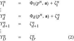
here a are the unknown parameters in the representation, D is the total number of PCs, are the residuals, which are assumed to be Gaussian and uncorrelated. So, for the reconstruction of this director mode, we should find the appropriate values ​​of the two latent variables p^m and parameters a. Note that it is easy to show that in the particular case of linear Φ this corresponds strictly to the traditional EOF rotation: minimization of the squares of the residuals under condition | a| = 1 gives the largest EOF in the a vector and the corresponding PC in p time series.

Within the framework of the Bayesian paradigm, the cost function used for training the model (2) is constructed as a probability density function (PDF) of unknown variables under the condition of dataX¹, …, X^NOT: the learning model (2) consists in finding the global maximum of this PDF on unknowna and p¹, …, p^NOT. This PDF can be expressed by Bayes’ theorem:

here P(X¹, …, X^NOT| a, p¹, …, p^NOT): = THE( a, p¹, …, p^NOT) is a likelihood function, i.e. the probability that the data X are obtained both by the model (2) with the parameters a and the series p¹, …, p^NOT and the subsequent rotation by matrix V. This function can be easily written under the assumption of normality and whiteness of noise (see Additional Methods for details); its maximum is reached for minimum mean squared errors of. But the crucial point is the specification of a priori information, which reflects all the desirable properties of the solution, in the form of a priori probability densities of a and p¹, …, p^NOT.

The main a priori the assumption we suggest to use is the dynamic nature of the hidden mode p time series; in other words, we need every running point p^m be connected with the previous one p_m-1. Namely, we introduce a prior probability density for p¹, …, p^NOT in the following form:

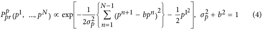
In fact, Eq. (4) determine a preliminary set of p time series made up of various realizations of colored noises so that most of them have a self-correlation time . The second condition of (4) provides the a priori unitary variance of eachp^m~ NOT(0, 1). Although the set thus defined is fairly general, it provides an efficient restriction on the class of possible solutions by excluding short-scale signals from consideration.

Under the a priori constraint (4) we have introduced a representation of the functions Φ (.) In (2) as a superposition of polynomials Π_I( p) which are mutually orthogonal in the probability measure defined by (4):

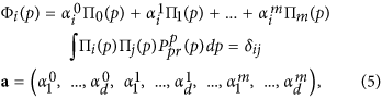
or_I is the Kronecker Delta. Such a representation considerably facilitates a procedure of learning the model, since the problem becomes linear with respect to the parameters. a. At the same time, it increases the power of the model by simply adding more orthogonal polynomials in (5). The idea of ​​defining a PDF a priori for the parameters of such a representation is quite obvious: it should be the most general functions, but allowing Φ_I(.) to get a priori the same variances as the corresponding time series of PC Yes_I (correlations between different PCs Yes_I are zero, so we don’t need to worry about covariances). Thus, it is reasonable to define this PDF as a product of Gaussian functions of each with gap , where.〉 denotes the mean over time. The same parameter restrictions were used, for example, in^34.35 concerning the outer layer coefficients of artificial neural networks used to adjust an evolution operator.

Optimal model selection

It is clear that the proposed method provides a solution which strongly depends on three parameters: D – the number of PCs involved in the nonlinear transformation, m – the number of orthogonal polynomials determining the degree of non-linearity and – the autocorrelation time characteristic of the reconstructed mode. All of these values ​​determine the complexity of the data transformation and therefore should be relevant to the statistics available. For example, if we take a very large m and = 0, we would obtain the curve passing through each point and our unique mode p¹, …,p^NOT would capture all the variability in the subspace of the D first PCs. But, indeed, in this case, we would get an overfitted and statistically unjustified model. Thus, an optimality criterion is necessary allowing the selection of the best model among the set of models defined by different values ​​of ( D,m,). We define optimality E by a Bayesian proof function, i.e. the probability density of the data X¹, …, X^NOT given the model ( D,m,):

Really, E is the minimum amount of information needed to transfer the given series Yes¹, …, Yes^NOT by the model ( D, m,); thus, the same criterion could be derived within the framework of the principle of minimum description length³⁶). The model corresponding to the smallest E, or, which is the same, providing the maximum probability of reproducing the observed time series, is considered optimal.

The Bayesian proof function can be calculated by the likelihood integral on all parameters a and latent variables p¹, …, p^NOT with the a priori probability measure:

We compute this integral by the Laplace method by supposing that the principal contribution comes from the neighborhood of the maximum of the integrand on all the variables; see details in additional methods. The possible optimality can be expressed in the following form:

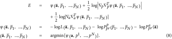
here are estimated values ​​corresponding to the minimum of the function ψ (.) – minus log of the cost function; and designate the operators of second derivations on allp^m and a Consequently. The last two terms of (8) penalize the complexity of the model; they ensure the existence of an optimum of E on all models. Thus, to estimate the optimality of the given model with ( D, m, Ï„), we should (i) learn the model by finding the values then (ii) calculate the penalty terms as determinants of ψ (.) second derivation matrices in the parameter domains a and latent variables p¹, …, p^NOT in the tip .

Main steps of the algorithm

The main steps of the proposed algorithm are as follows.

1. 1

   Data data rotation to PCs : Yes^m= V^TX^m; columns of theV matrix are EOFs of theX time series.

2. 2

   Find the optimal model in the PC spaceYes. This step includes the search for the optimal dimension D of the subspace for a nonlinear expansion, estimation of the optimal degree of nonlinearity m as well as the autocorrelation time characteristic of the hidden mode. Here we also get concrete parameters optimal mode.

3. 3

   Subtract the obtained mode corresponding to the maximum of the cost function of the data vectors:

   

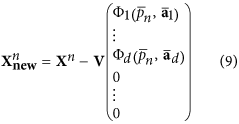
   The vector of the mode image obtained in the PC space is completed by D – D zeros, since only D PCs are involved in nonlinear transformation. In fact, at this step, we define the new data vectors – the residues between the initial values ​​and the values ​​of the mode. After that we will find the following mode: the same procedure from i.1 is applied to new data .

The iteration of procedure i.1 – i.3 is stopped when one obtains time series p of the new mode equal to constant zero, or, equivalently, we find that the optimal degree m of polynomials (5) is zero. This means that we can no longer resolve nonlinearities in the data and the noise is most likely significant; in other words, the best we can do is a traditional EOF decomposition of the residues. In particular, the expansion of the SST time series into three NDMs presented in this document gives D= 5, m= 3 for the first NDM, D= 4, m= 6 for the second andD= 8,m= 8 for the third. Finally, the set of nonlinear expansion of the data can be written as follows:

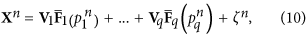
orqis the total number of NDMs obtained. Note that each of the NDMs is defined in its own subspace, which is rotated with respect to the initial data space: the orthogonal matricesV_I are different for different NDM.